Extract insights from tag lists using Python Pandas and Power BI


Tag lists provide a flexible means of capturing information, but can often make it difficult to extract valuable insights from the data.
To illustrate how to tackle this challenge, we will process the Star Wars dataset from Kaggle.
We use a number of technologies:
- Python Pandas for the data wrangling. The name Pandas is derived from "panel data".
- Microsoft Power BI to load the output from Pandas, to create a semantic model and to apply analytics.
We find this to be a powerful combination of technologies for many data analytics applications. In particular where we want to generate insights from data sources such as CSV files and spreadsheets where the data volumes are in the order of Megabytes rather than Gigabytes.
Step 1 - load and prepare the data using Pandas
The first step involves importing the Pandas package and using that to load the data into a dataframe. A dataframe is used to capture tabular data, it comprises rows and columns and is similar to Excel worksheets and Databases tables.
We are focusing on the planets.csv file which you can download from Kaggle here. It contains a listing of 61 planets. Having downloaded the file locally, we use the following Python code to load the data from CSV into a Pandas dataframe. We then inspect the first 5 rows of data using the head() method.
import pandas as pd
planets = pd.read_csv("../data/raw/kaggle-starwars/planets.csv")
planets.head(5)
| id | name | rotation_period | orbital_period | diameter | climate | gravity | terrain | surface_water | population |
|---|---|---|---|---|---|---|---|---|---|
| 0 | Alderaan | 24.0 | 364.0 | 12500.0 | temperate | 1 standard | grasslands, mountains | 40.0 | 2.000000e+09 |
| 1 | Yavin IV | 24.0 | 4818.0 | 10200.0 | temperate, tropical | 1 standard | jungle, rainforests | 8.0 | 1.000000e+03 |
| 2 | Hoth | 23.0 | 549.0 | 7200.0 | frozen | 1.1 standard | tundra, ice caves, mountain ranges | 100.0 | NaN |
| 3 | Dagobah | 23.0 | 341.0 | 8900.0 | murky | NaN | swamp, jungles | 8.0 | NaN |
| 4 | Bespin | 12.0 | 5110.0 | 118000.0 | temperate | 1.5 (surface), 1 standard (Cloud City) | gas giant | 0.0 | 6.000000e+06 |
On inspection of the dataframe above, we can see that the terrain column is a string, which contains comma separated categories. For example, the planet Hoth has three categories tundra, ice caves, mountain ranges whereas Dagobah has two swamp, jungles.
We now take a look at the general composition of the planets dataframe using the info() method.
planets.info()
RangeIndex: 61 entries, 0 to 60
Data columns (total 9 columns):
  #   Column           Non-Null Count  Dtype
---  ------           --------------  -----
  0   name             60 non-null     object
  1   rotation_period  48 non-null     float64
  2   orbital_period   48 non-null     float64
  3   diameter         44 non-null     float64
  4   climate          48 non-null     object
  5   gravity          44 non-null     object
  6   terrain          54 non-null     object
  7   surface_water    26 non-null     float64
  8   population       43 non-null     float64
dtypes: float64(5), object(4)
memory usage: 4.4+ KB
We can see that we have 8 columns, across 61 rows. However, we also note that one of the rows appears to be empty (61 entries, but 60 non-null entries in the name column).
The powerful .loc[] method is used to display the rows where the planet name is null.
planets.loc[planets.name.isna()]
| id | name | rotation_period | orbital_period | diameter | climate | gravity | terrain | surface_water | population |
|---|---|---|---|---|---|---|---|---|---|
| 26 | NaN | 0.0 | 0.0 | 0.0 | NaN | NaN | NaN | NaN | NaN |
So we drop row this from the data set:
planets.dropna(axis=0, subset="name", inplace=True)
Finally, we rename the name column to planet_name to make things easier to follow later on in the process:
planets.rename(columns={"name": "planet_name"}, inplace=True)
Step 2 - parse the terrain column using split method
The next major step is to convert the unstructured data in the terrain column into structured data by parsing it as a set of comma separated strings. We note that each category is separated by a comma and a single space, so we use this as the argument for the str.split() method, applying it to the terrain column as follows:
planets["terrain"] = planets["terrain"].str.split(', ')
planets["terrain"].head(5)
0                 [grasslands, mountains]
1                   [jungle, rainforests]
2    [tundra, ice caves, mountain ranges]
3                        [swamp, jungles]
4                             [gas giant]
Name: terrain, dtype: object
This results in the terrain column containing a list object rather than a string object.
Step 3 - create bridge table by applying the explode method
Now that the terrain column contains an iterable object, we can exploit this by applying the explode() method to the planets dataframe to create a new planet_terrain_bridge dataframe:
planet_terrain_bridge = planets.explode("terrain")
planet_terrain_bridge
| id | planet_name | rotation_period | orbital_period | diameter | climate | gravity | terrain | surface_water | population |
|---|---|---|---|---|---|---|---|---|---|
| 0 | Alderaan | 24.0 | 364.0 | 12500.0 | temperate | 1 standard | grasslands | 40.0 | 2.000000e+09 |
| 0 | Alderaan | 24.0 | 364.0 | 12500.0 | temperate | 1 standard | mountains | 40.0 | 2.000000e+09 |
| 1 | Yavin IV | 24.0 | 4818.0 | 10200.0 | temperate, tropical | 1 standard | jungle | 8.0 | 1.000000e+03 |
| 1 | Yavin IV | 24.0 | 4818.0 | 10200.0 | temperate, tropical | 1 standard | rainforests | 8.0 | 1.000000e+03 |
| 2 | Hoth | 23.0 | 549.0 | 7200.0 | frozen | 1.1 standard | tundra | 100.0 | NaN |
| ... | ... | ... | ... | ... | ... | ... | ... | ... | ... |
| 57 | Kalee | 23.0 | 378.0 | 13850.0 | arid, temperate, tropical | 1 | canyons | NaN | 4.000000e+09 |
| 57 | Kalee | 23.0 | 378.0 | 13850.0 | arid, temperate, tropical | 1 | seas | NaN | 4.000000e+09 |
| 58 | Umbara | NaN | NaN | NaN | NaN | NaN | NaN | NaN | NaN |
| 59 | Tatooine | 23.0 | 304.0 | 10465.0 | arid | 1 standard | desert | 1.0 | 2.000000e+05 |
| 60 | Jakku | NaN | NaN | NaN | NaN | NaN | deserts | NaN | NaN |
You can see from the output above that the explode() method repeats each row in the dataframe for each item listed in the original terrain column.
We now apply some steps to wrangle this new planet_terrain_bridge dataframe into a suitable form so that can act as a "bridge table". This table will be used to resolve the "many to many" relationship between planets and terrains. This is a common approach in data modelling that we will adopt in Power BI to generate analytics that are intuitive for end users:

First we trim the dataframe down to the two columns we need: planet_name and terrain. We use the loc[] syntax to do this:
planet_terrain_bridge = planet_terrain_bridge.loc[:, ["planet_name", "terrain"]]
planet_terrain_bridge.reset_index(drop=True, inplace=True)
planet_terrain_bridge
| id | planet_name | terrain |
|---|---|---|
| 0 | Alderaan | grasslands |
| 1 | Alderaan | mountains |
| 2 | Yavin IV | jungle |
| 3 | Yavin IV | rainforests |
| 4 | Hoth | tundra |
| ... | ... | ... |
| 147 | Kalee | canyons |
| 148 | Kalee | seas |
| 149 | Umbara | NaN |
| 150 | Tatooine | desert |
| 151 | Jakku | deserts |
We then note that some of the planets (such as "Umbara" above) do not have a terrain category applied. So we drop these rows from the dataframe using the dropna() method to vreate the final dataframe.
planet_terrain_bridge.dropna(axis=0, subset="terrain", inplace=True)
planet_terrain_bridge
| id | planet_name | terrain |
|---|---|---|
| 0 | Alderaan | grasslands |
| 1 | Alderaan | mountains |
| 2 | Yavin IV | jungle |
| 3 | Yavin IV | rainforests |
| 4 | Hoth | tundra |
| ... | ... | ... |
| 146 | Kalee | cliffs |
| 147 | Kalee | canyons |
| 148 | Kalee | seas |
| 150 | Tatooine | desert |
| 151 | Jakku | deserts |
Step 4 - create a terrains table
We do not have a master data resource for terrains, so we will create our own by generating a list of the unique terrain codes found in the data.
list_of_terrains = list(planet_terrain_bridge["terrain"].unique())
list_of_terrains.sort()
terrains = pd.DataFrame.from_dict({"terrain": list_of_terrains})
terrains.head(5)
| id | terrain |
|---|---|
| 0 | acid pools |
| 1 | airless asteroid |
| 2 | ash |
| 3 | barren |
| 4 | bogs |
We can see some immediate opportunities to consolidate the list of terrains. For example, singular / plural duplicates exist for six terrains:
for terrain in list_of_terrains:
    plural_terrain = f"{terrain}s"
    if plural_terrain in list_of_terrains:
        print(f"{terrain} and {plural_terrain}")
desert and deserts
jungle and jungles
mountain and mountains
ocean and oceans
savanna and savannas
swamp and swamps
But we'll save these steps for a future blog post!
Step 5 - write output to file
Now we write the planets data minus the terrain column and the new bridge and terrain dataframes to CSV file so that we can load it into Power BI for analysis.
planets.drop(labels="terrain", axis=1).to_csv("../data/output/starwars-planets/planets.csv", index_label="planet_id")
planet_terrain_bridge.to_csv("../data/output/starwars-planets/planet_terrain_bridge.csv", index_label="planet_terrain_bridge_id")
terrains.to_csv("../data/output/starwars-planets/terrains.csv", index_label="terrain_id")
Step 6 - load data into Power BI
Load all three CSV files into Power BI as UTF-8 commma delimited text / CSV files. Promote the first row as headers in all cases if this is not done automatically by Power BI.
Once loaded, set up the Model in Power BI so that the planet_terrain_bridge table resolves the many to many relationship as follows:
- A one to many relationship between planets[name] and planet_terrain_bridge[name]
- A one to many relationship between terrain[terrain] and planet_terrain_bridge[terrain]
This should look as follows:
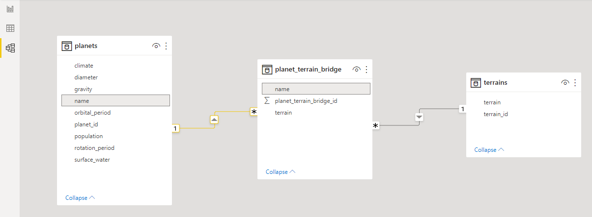
Finally we decide to hide the planet_terrain_bridge in the report view - this is because we do not want end users to use data from this table in reports directly:

Step 7 - create new measures
Next we unleash the "power" in Power BI, by creating measures that will calculate results dynamically as users interact with Power BI visuals and filters. These are written in DAX which appears at first to be similar to formulas you may write in an Excel spreadsheet. However, DAX is specifically designed to work with tabular data, and therefore is able to unlock significant value from data held in the Power BI model by generating new insights.
In this case, we create two new measures as follows:
The first measure Terrain Count counts the number of unique terrains in the planet_terrain_bridge table for the given filter context. The use of COALESCE will ensure that the result returns 0 rather than BLANK if the report is filtered to a planet (or set of planets) that do not have a terrain associated with them through the bridge table (there are six of these).
Terrain Count = COALESCE(DISTINCTCOUNT(planet_terrain_bridge[terrain]), 0)
The second measure Planets With Terrain Count takes the same approach as Terrain Count but counts the number of unique planets in the planet_terrain_bridge table for the given filter context. Again coalesce plays a role by returning 0 if the report is filtered to a terrain (or set of terrains) that do not apply to a specific planet:
Planets With Terrain Count = COALESCE(DISTINCTCOUNT(planet_terrain_bridge[planet_name]), 0)
Step 8 - create visualisations
The final step is to create interactive visualisations using the Power BI model and measures created above.
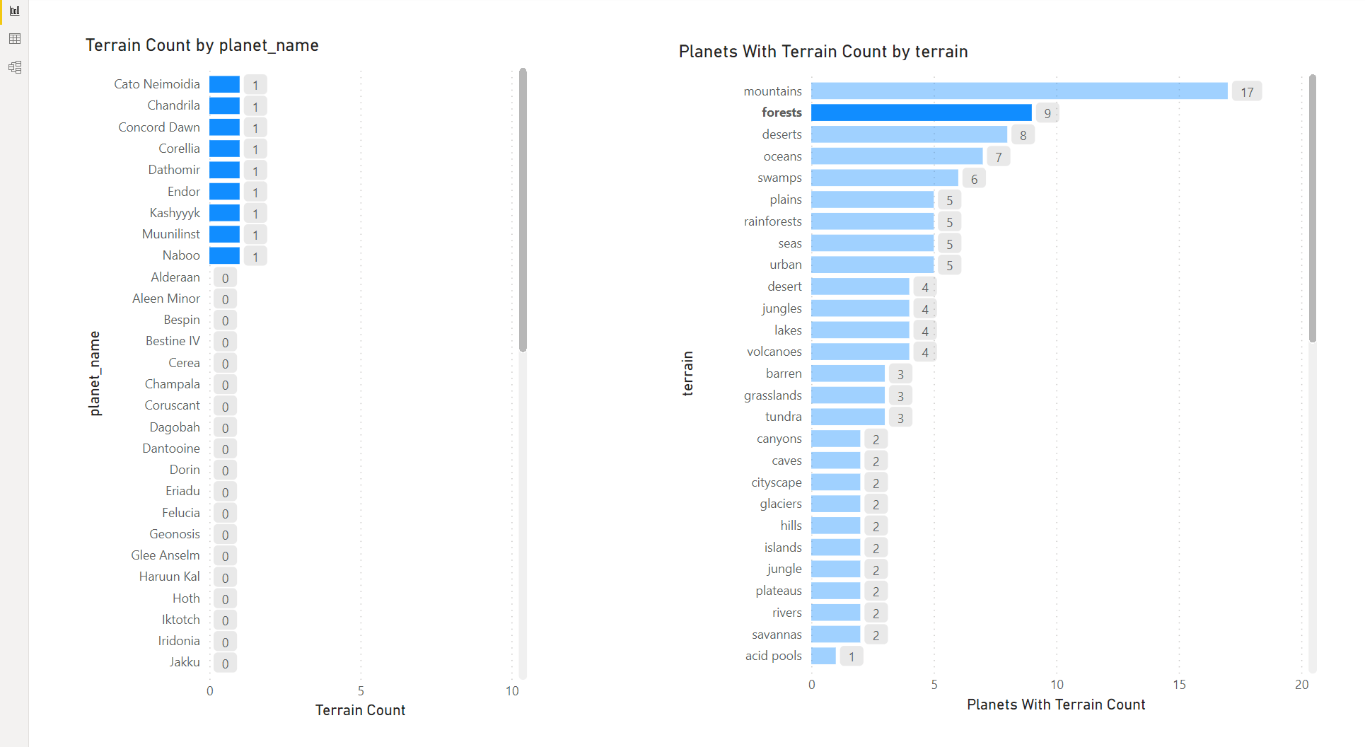
First, create a stacked bar chart that shows the count of terrains for each planet as follows:

Next, create a stacked bar chart that shows the count of planets for each terrain category as follows:

Arrange these visuals side by side on the page as follows:

Interacting with either chart causes the other to filter. This starts to unlock the value from the data - for example, if a user wants to explore how many planets have a terrain category of forests, they select this category on the right hand chart, and the left hand chart is filtered accordingly:
Conclusions
We have set out the basic steps that can be taken to unlock value from data that has been captured as a tag list.
This is based on:
- Using the Pandas Python package to load the raw data into a datframe.
- Inspecting the contents of the datframe and performing any data clean up steps as required.
- Using two Pandas methods
str.split()andexplode()to process the column containing the tag list - transforming it from unstructured data to structured data. - Using the exploded dataframe to create a "bridge" table to resolve the many to many relationship between the primary entity (planets) and the tag categories (terrains).
- Setting up a model and measures in Power BI that exploit the presence of a bridge table.
- Creating interactive visualisations that enable end users to explore this data in an intuitive way, allowing them to answer questions that would not have been possible without taking the steps above.
We have also uncovered some of the practicalities of working with data of this nature:
- There is generally a need to clean and prepare data before you can do something meaningful with it! The scale of data ingestion, cleaning and transformation work should not be underestimated, it is not unusual for this type of work to consume circa 60% to 80% of the total effort associated with a data project. The Pandas package provides a rich set of methods to help perform these steps.
- With no master data resource for the terrain categories, we were required to build our own from the data to hand. But what if there was a terrain category that did not appear in this specific data set? For example, would it be useful to show that no planets were present that had a terrain type of "marsh"?
- We also highlighted a number of cases where the terrain categories themselves could be consolidated. For example we have 6 terrains that are duplicated in both singular and plural form. Can we automate this process without having to hand craft each such correction / consolidation?
Finally, we haven't applied engineering practices that are essential if the solution was being put into use at scale in a production environment:
- How can we protect from unanticipated changes to the source
planets.csvfile? - How can we verify that the requirements are being met?
- How can we publish the output to cloud storage so that the Power BI Service (rather than Power BI Desktop) can access it?
- How can we deploy this functionality to a cloud resource and automate running it?
- How could we scale up the solution if the data being processed was in the order of Gigabytes or even Terabytes?
These are all questions that I will aim to tackle in future blogs.
Credits
Many thanks to Joe Young for publishing the Star Wars dataset on Kaggle.